Basic
Option Pricing
by
Rich Tanenbaum
(from Topics
in Money and Securities Markets, Bankers Trust Company, Money
Market Center, June 1987.)
INTRODUCTION
This paper
presents several simple but powerful methods for valuing options.
A discussion of options appears in Topics in Money and Securities
Markets, "A Framework for Understanding
Options: Defining Their Payoffs and Risks"
This piece
will draw upon the concepts introduced there to develop two straightforward
and intuitive pricing methodologies. It will then derive a more
rigorous and sophisticated technique using basic mathematics,
and finally will demonstrate how the three are related to each
other.
AN
EXPECTED VALUE ARGUMENT
A
Game.
First, let's
consider a game. A coin is going to be flipped. If it comes up
heads, you will receive a dollar. If it comes up tails, you will
receive nothing, nor will you pay anything. To play the game,
though, you must pay a fee. How much are you willing to pay? Certainly,
you would be stupid to pay more than a dollar. And anybody would
play for free. Between these two bounds, though, there are 99
different prices (rounded to the nearest penny), and any of them
are plausible. The amount an individual pays will be function
of what he feels comfortable with. We call this his level of risk
aversion. If you are very cautious, you won't pay too much for
the game. You don't like the idea of losing the fee, even in the
face of a large potential profit. If you seek risk, and you get
a thrill just from playing, regardless of the outcome, you might
be willing to pay quite a lot. Then again, you could be risk neutral.
This puts you right in the middle, in that you do not shy away
from risky situations, nor do you go out of your way to find them.
Risk neutral
players assess the probability of each outcome, heads and tails,
and calculate the expected payoff from the game. In this case,
you would calculate that you would expect to be given 50 cents,
since there is a one-half probability of getting a dollar, and
a one-half probability of getting nothing. While there is absolutely
no chance of receiving 50 cents at the end of the game, that is
the one best guess of what you will have. Based on this expectation,
paying anything less than 50 cents to play will leave you with
an expectation of making money from the game, and paying anything
more than that will leave you with an expectation of a loss. You
would, therefore, pay any amount up to and including 50 cents.
Let's look
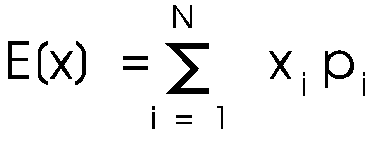
at the expected value formula a little more closely. If we have
a set of N possible outcomes, each denoted x1,x2,...xN the equation
for the expectation of x, denoted E[x] is:
 {1}
{1}
where pi is
the probability of achieving xi.
This formula
is a lot like the one for the average of a bunch of things. Instead
of adding things up and dividing by the number of things you added,
you add up the product of each thing times the probability that
the thing will happen. The standard average is actually a special
case of the above formula, where the probability of every event
is equal to the probability of every other event. This implies,
since the probabilities must sum to one, that each probability
is equal to 1/N. Another term for the expectation is the weighted
average.
In our game,
a risk neutral player would calculate the fee he'd be willing
to pay by taking the weighted average of the payoffs:
1(.5) + 0(.5)
= .5
Another
Game
Let's suppose
now that the game is played a little bit differently. As before,
a fee is paid to play. This time, though, the coin isn't flipped
for another year. This means the player has to wait a year to
get a dollar, if the coin comes up heads. What will a risk neutral
individual pay for this game?
If we proceed
as before, we would again get 50 cents. But this really represents
what she would pay if she could get into the game in a year, not
today. Since one must pay today, it's only fair to pay just the
present value of the fee that would be paid in a year. She'll
need to determine the appropriate rate to discount the payoff.
If she doesn't trust the person running the game to fulfill their
promise to pay off if she wins, then she may want to use a very
high rate. If she has some sort of a guarantee of payment, it
seems reasonable to use the rate that she could earn on an alternative
risk free investment (where free refers to the lack of any default
risk). One possible instrument is a one year U.S. Treasury bill,
since she trusts the government to honor its debt, and one year
is the period over which she will discount. We will refer to this
as the one year risk free rate. If this rate is 10% per year,
then the risk neutral player would pay up to 45 cents for this
new game (since fractional pennies don't count).
A
Third Game, For Review.
What if the
game was based on the roll of a die? Your payoff is the number
on the die squared. Thus, if the number three comes up, you get
$9. The expected payoff of the game is:
1(1/6)+4(1/6)+9(1/6)+16(1/6)+25(1/6)+36(1/6)=
15.17
If the die
isn't rolled for a year, then the risk neutral player will pay
the present value of $15.17 to play the game.
With all this
math, you might be asking a basic question: who cares about the
risk neutral player? You might be risk neutral yourself, or someone
you know could be, and that's reason enough. Even if you don't,
it turns out that the math is much easier when we concern ourselves
with these people So consider yourself lucky.
Applying
the Expected Value Argument to Options
Another basic
question you might be asking is: What does all this have to do
with options? Well, let's talk about yet another game...
Instead of
flipping a coin, or rolling dice, you are offered a game based
upon the closing price of a stock the last Friday of next month.
Instead of the payoff being 0 or 1, and instead of it being the
stock price squared, we'll make it one dollar for every point
the stock is trading over 100. If the stock is below 100 that
day, you won't get anything. Once more, how much would a risk
neutral player be willing to pay to get into this game?
The most obvious
thing to do at this point is apply the same reasoning used above:
calculate the expected payoff of the game. If we consider only
integer values of the stock, and denote the stock price as S,
and the probability that the stock price ends up with the value
x as p(x), the formula for the expected value of the cash payoff,
E[C], is:
 {2}
{2}
It turns that
E[C] is very much like the price a risk neutral investor would
pay for a call option on S with a strike of 100, the only difference
being that the payoff of the call must be discounted to the present.
We could start
the summation at S=0 instead of S=100. In that case, our payoff
would be max(0,S-100). Each way yields the same answer.
There are
a few problems with this formula. First, the stock can hit more
prices than just the integers. We can consider finer gradations,
but it won't change the value much. We will also take a long time
to do this calculation if we consider all the prices between 100
and infinity. If the probability of very high prices is very small,
approaching zero, then we can ignore movements in the stock to
prices that are above some actual threshold. We can also work
with higher and higher underlying values until the price of the
option doesn't change very much when we add the next term. In
this way, the formula above may be modified to work well with
the particular option we are interested in valuing.
Another problem
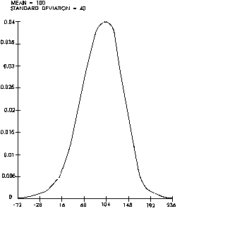
is what probabilities to use. One of the simplest assumptions
is that the stock price is normally distributed, which says any
price is possible, but the price will most likely be close to
some middle value, or to the expected value. A graph of a normal
distribution is shown in Figure 1, where we can interpret the
x axis as, say, the level of the stock price in three months.
Notice that
prices nearer to today's prices are more likely. However, there
is some probability (however small) that the price can go negative.
This is very unrealistic. Just as no one would be able to buy
our games for less than zero, no one would be willing to sell
a stock for less than zero (barring things like lawsuits that
will send all owners as of the trial date to jail, when the trial
hasn't started yet).
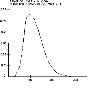
Our way around
this will be to assume that the stock is lognormally distributed.
This means that if we take logs of the stock prices and put them
on the x axis, we will get a curve with the same shape as Figure
1.
Figure
1. Normal Density Function For A Stock at 100
The graph
of the lognormal distribution is shown in Figure 2.
Figure
2. Lognormal Density Function For A Stock at 100
Given this
picture, we can calculate the probability of hitting each stock
price. One way to do this is to draw Figure 2 on very fine graph
paper, and count the number of covered boxes between two prices.
Dividing this by the total number of covered boxes will yield
the probability that the price of the stock will fall in that
range. A simpler way to do it is to look up the probability in
a normal distribution table. (Since the normal curve is such a
common function, tables have been created for it. Since tables
have been created for it, it is a commonly used function.) If
you believed that the probability distribution looked different
from a normal curve, you could still draw your own, and count
boxes. It's tedious, but it's a nice technique to fall back on.
Applying either of these two (2) gives us an option pricing formula.
It's worth
noting that this is a way to perform integration. Integration
is the technique from calculus where one calculates the area under
a curve. This amounts to a mathematical method for counting boxes,
where the boxes are infinitesimally small.
Using
payoff diagrams
Formula 2
is a special case, because we knew the game only had value when
the stock was worth more than 100 at the end. The part of the
formula where we took S-100 was particular for a 100 strike call.
By using payoff diagrams, we can generalize the formula.
One type of
option payoff diagram is a graph of option profit or loss versus
the underlying asset's value of the option itself, rather than
profit or loss (the difference between the two graphs is that
one subtracts the option premium and the other doesn't).
The payoff
diagram of a call option with a strike price of 100 is shown in
Figure 3.
Figure
3. Payoff Diagram of a 100 Call
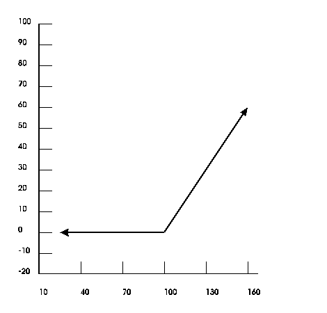
This represents
graphically the option being worthless at expiration if the underlying
is trading at less than the strike, and worth intrinsic value
(underlying price minus strike price) otherwise. In equation (2),
we took a weighted average of max(O.S-100). In effect, we calculated
the weighted average of the option payoff. By using the payoff
diagram, we can restate (2) as:
 {3}
{3}
We now have
a general method for valuing options, or at least determining
what a risk neutral investor would be willing to pay for them.
First, we construct a payoff diagram. Then, we assume a probability
distribution, and calculate the expected payoff. The only step
we've left out is the present value effect. We need to discount
this expected value back from the option expiration to the present,
using the appropriate risk free rate.
SIMULATION:
ANOTHER WAY TO DO EXPECTED VALUE
When
you don't want to count boxes
While the
method of calculating the expected payoff of an option described
above is perfectly adequate for many situations, there will be
times when we (1) don't know the underlying asset's probability
distribution, (2) know it but cannot conveniently express it,
or (3) don't want to spend time counting little boxes. Simulation
is a technique which, in the current context, allows us to artificially
create many different market movements, and then claim that the
movements observed capture virtually all the future possibilities.
As such, it can save from the above three problems.
To create
an option value via simulation, we start our underlying asset
out at its current price, and then randomly generate a price change,
or return, for it. Let's say we produce weekly returns. First,
we generate a random return for the first week. Then we generate
another return, until we have gotten a return for every week the
option has until expiration. If it was a one year option, we'd
generate 52 returns. We will then have a prospective price for
the asset at the end of the year, and can determine the intrinsic
value of the option given that price. We note the value, and then
start the process over again, generating 52 more returns, and
so on. After doing this 1000 times, we will have 1000 intrinsic
values, each of which occurred one time out of a thousand. The
only steps left are to take the average of these thousand intrinsic
values, and discount it back to the present at today's one year
rate. The averaging is simpler than that done in section 2, since
the probability of each event is one out of a thousand; we can
just add our thousand intrinsic values and divide the sum by a
thousand.
As before,
we have total freedom to choose the distribution of random numbers.
Besides normal and lognormal, such esoteric processes as truncated
normal, beta, gamma, and others are possible. As long as we can
generate random numbers that conform to a given distribution,
we can simulate option values by assuming the underlying asset
follows that process.
If this was
all the simulation was good for, however, we would only be solving
our third dilemma, avoiding the tedium of counting boxes. There
are two other types of distributions we are going to examine for
which simulation may be necessary to value options, and not just
convenient. The first of these is a class we shall call "contaminated
distributions," used here to illustrate our second problem
stated above. These are any combination of simpler distributions.
For example,
we can assume an asset's returns are generated lognormally, but
that the variance of the process changes over time in a non-deterministic
fashion. In one week, the variance could be 10%, and the next
week 25%. The level of the asset's variability is a function of
some other random number, which could, for example, be uniformly
distributed. (The uniform distribution is one in which every number
within the upper and lower bounds has equal probability.) In other
words, we first pull a random number from a distribution with
bounds 0 and 1, such that if the number is less than .8, the asset's
variance is 10% that week, and if the uniform number is above
.8 the asset's variance is 25%. The following week the uniform
number is drawn again, so that over time the asset's movement
might appear stable for awhile, and suddenly jump wildly. While
this particular return generating process might be reducible to
a simple probability distribution, one would need a fairly sophisticated
statistical training to perform the transformation. Simulation
provides a much easier way to do this and, if enough simulations
are run, an equivalent way, as well.
Another type
of simulation we can run uses the "bootstrap method."
This also generates random returns, but uses actual data instead
of solely employing a random number generator. To bootstrap, we
first take a series of historical returns, and put them all in
a hat. We then randomly pull one out, and that is our return for
the first period. The number is put back in the hat, so that we
are always pulling rorm a hat that contains the same returns.
We pull another return from the hat, and that becomes the return
for the second period. We continue this way until we've gotten
a return for each period in the options life.
The advantage
of this method is that we don't have to make many assumptions
about the underlying asset's return distribution, we just let
the chips fall where they may. We aren't totally free from having
to make any decisions, though. In particular, it is necessary
to state whether the returns we are pulling out are rates of change,
or actual changes (i.e., does the asset follow a multiplicative
or additive random walk). We also want to pick a time period which
we believe is relevant for forecasting the future changes in the
asset. In addition, we must assume that the underlying returns
from different points in time are independent of each other. On
the whole, though, it is a much less stringent method of simulation,
and comes closer to solving the first problem above: knowing the
underlying asset's probability distribution.
Note that
the simulation approach, whether bootstrapped or not, is very
similar to the first pricing method discussed in this paper, that
of applying the underlying asset's probability distribution to
a simulation of all possible intrinsic values. In the long run,
a simulation ought to yield the same answer as that approach.
The reason for this is that we are still sampling values form
the supposed underlying distribution, and taking an expectation
of the intrinsic values. With simulation, we hope that drawing
a large amount of random numbers will give us a set of intrinsic
values which occur with the proper frequency, while summing over
the entire distribution guarantees it. If we don't know the distribution,
but have the data, we can bootstrap where we can't sum. Then again
the summation is faster. To gain an appreciation for the trade-offs
between the two approaches, later on we shall present some option
values using each method.
It is nice
that we have an intuitive way to value as complex a security as
an option. It is unfortunate that we not only need to estimate
the probability that the underlying asset will move a certain
amount, but also assume investors are all risk neutral. The next
section will present a slightly more sophisticated model which
alleviates this situation.
THE
BINOMIAL MODEL, IN FOUR EASY STEPS
Assumptions
For the purposes
of the model presented here, we are going to make a number of
simplifying assumptions. Many of these can be relaxed quite easily,
but that is beyond the scope of this paper. We will first state
that we are valuing a
- three month
- European
(exercise allowable only at expiration)
- call option
- with a
strike price of 100
- on an asset
which pays no cash over the life of the option.
We assume:
- The underlying
asset can be bought and sold in any quantity
- without
any transactions costs,
- taxes or
- penalty
for short sales.
- We can
borrow and lend freely at the risk free rate.
- This risk
free rate is assumed to be known and constant over the life
of the option (we'll use .5% per month here).
- The underlying
asset can only go up or down over discrete periods,
- in an amount
that is known and constant over the life of the option.
All but the
last seem fairly standard, simplifying assumptions. The last one
requires an explanation. One example of a price process that follows
this path is a stock that is trading at 1200 today, and next month
its price can either go up to 102 or down to 98. If it goes to
102, then one month after that it can either go up to 104 or back
down to 100. If the price next month is instead 98, then the next
month will see the price back at 100 or down to 96. Notice that
we are not allowing the price to stay the same from period to
period, nor to take on a richer set of values.
Step
1: Build a tree
The first
thing we want to do is represent the prices of the previous paragraph
pictorially. A tree structure is a convenient way to do this,
and it is demonstrated in Figure 4.
Figure
4: A Tree of Possible Underlying Values
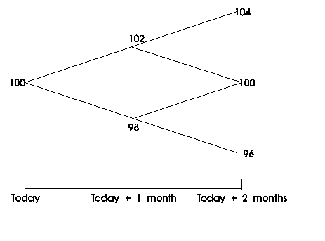
Given a starting
price of 100, we can specify every possible path over the next
few months. The tree does not get too "bushy," since
two periods hence there are only three values instead of four.
This arises from the fact that going down and then up is the same
as going up and then down. This is partly a function of the jump
sizes being constant over time, as was assumed above.
If we propagate
this structure very far out (51 months, to be precise) we will
notice a problem encountered earlier. After 51 down moves of two
points each, the price of the underlying asset will be -2. What
we need to do is specify our jumps as multiplicative changes,
rather than additive. Let's make an up move (call it U) equal
to 1.02 times the price in the previous node, and a down move
(call it a d) equal to the price times .98. Then, after 51 periods,
our smallest value will be 35.69 {100(.98)(.98)(.98)...with .98
repeated 51 times; the same as 100(.98 to the power of 51)}, well
above 0.
Notice that
this preserves the clean tree we had earlier, since an up down
will yield a price after two periods that is equal to a down up:
100(1.02)(.98)
= 99.96
100(.98)(1.02)
= 99.96 {4}
While this
is nice, it's a bit unsettling that there will be this downward
drift in the tree, losing .04% of value every two periods. We
need to be careful, though. If we assign a high enough probability
that u will be realized, the expectation of the price next period
could still be as high as S(u).
Even though
the probabilities can perhaps compensate for this downward drift,
we will still need to impose the constraint that u be greater
than one plus the risk free rate, and d less than one plus the
risk free rate. The reason for this is quite simple. Suppose the
money it costs to buy the underlying asset could instead be invested
at the risk free rate, and this rate is higher than both u and
d. This implies that the underlying asset will always underperform
the riskless asset. We say then that the risk free asset dominates
the underlying asset, and we should never see this occurring in
nature. By the same token, if the risk free rate is less than
u and d, it will be dominated by the underlying asset. Therefore,
one plus the riskless rate must lie between u and d. To value
a three month call with a strike price of 100, using u of 1.02
and d of .98 is consistent with a risk free rate of .5% per month,
or 6.17% annually. Our revised tree of possible prices now looks
like Figure 5.
Figure
5: A Tree of Possible Underlying Values Using Multiplicative Moves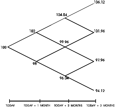
We can at
last proceed to the next step in pricing the option.
Step
2: Calculate the option value in the last period
The goal is
to determine the option price at the base of the tree, when the
underlying asset doesn't appear to be helping us at all. At expiration,
though, knowing the value of the underlying does tell us enough
to value the option. So let's look at the last part of the tree,
which is the set of possible underlying prices at the option's
expiration.
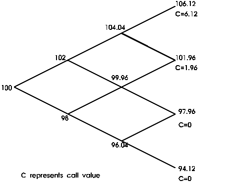
In the node
where the price is 106.12, we know the option will be worth 6.12.
We are not saying this node will definitely be reached, just what
the option will be worth if it is. Likewise, we can value the
option when the underlying is at 101.96. It will be 1.96. Doing
this for each node in the last period makes the tree look like
Figure 6, and we've started to value options.
Step
3: Set up the equivalent portfolio in the penultimate node
Unfortunately,
it's not quite that simple to get the next value. Fortunately,
it's not much more complicated. Let's go to the node in the second
to last period, where the underlying is worth 99.96. We know that
if the underlying asset goes up, the option will be worth 1.96,
and if it goes down the option will be worth 0. What we are going
to attempt now is to put together a portfolio, made up of a position
in the underlying and borrowing (or lending), that will be worth
1.96 when the underlying goes up, and nothing when the underlying
goes down. But how much underlying should we hold, and how much
to borrow or lend?
Rather than
guess, we can develop a couple of equations that state what we
would like. Suppose we buy D units of the underlying asset, and
borrow B dollars. We are going to borrow at .5%, as per our assumptions
above. The amount of money this portfolio will be worth if the
underlying goes up is:
101.96D -
1.005B {5}
In other words,
if D is .5, then owning half a unit of the underlying will have
a value of 50.98. Also, if we borrow $70, then we will have to
pay back $70.35. Likewise, if the underlying goes down, our portfolio
will be worth:
97.76D - 1.005B
{6}
What we are
trying to do is have the first equation be equal to 1.96, and
the second equal to 0. We thus have two equations to solve, with
two unknowns:
101.96 -1.005B
= 1.96
97.76D -1.005B
= 0 {7}
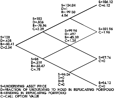
We can easily
find that D is .467, and B is 45.39. In other words, a portfolio
that has .467 units of the underlying, and borrows 45.39, will
give us the same payoff next period as the option will give us.
Applying the same type of dominance argument used earlier, we
conclude that this portfolio must cost the same amount as the
option does in the period we buy the portfolio. Since the outlay
to buy the underlying is .467(99.96)(which equals 46.65), and
we are taking in 45.39 from the borrowing, the net cash outlay
is $1.25. (We use the exact values of D and B to get this, not
the rounded values .467 and 45.39.) This is the cost of an option
with one period to expiration when the underlying is worth 99.96.
We can set
up the same equations in the other two nodes in that period, and
calculate option values for all three possible prices in two months.
Now let's go back one more month. The same calculation can now
be done, setting up a portfolio in that period that will be worth
the same amount as the option in the following period. For instance,
with the underlying at 98, we want to have 1.29 after an up move,
and 0 after a down move. Similar equations to the previous two
can be constructed:
99.96D - 1.005B
= 1.29
96.04D - 1.005B
= 0 {8}
We again solve
for D and B, and calculate the cost of that portfolio when the
underlying is trading at 98.
Step
4: Keep going back to today
We can then
go back another period, to today, and calculate the value of the
portfolio that will once again leave us with the same amount of
money as the option is worth. We will then be done, left with
the price of a three month call option. The full tree, with call
values, Ds and Bs filled in, is shown in Figure 7, where we calculate
the value of the option today, which is what we set out to do.
Figure
7 : A Tree of Underlying Prices, Call Option Values and the Replicating
Portfolio
(Strike =
100, Riskless Rate = .005%/period)
Interpreting
D and B
In every node,
we have a portfolio consisting of the underlying asset and borrowing
that will have the same value as the option in that node, as well
as in the nodes that can be reached in the following period. If
we like, we can also flip the portfolio over on its head, selling
D units of the underlying, and lending out some money. This will
cause us to have no cash flow in the next period, since whatever
positive value the option has, the portfolio will have an equal
but negative value.
The usefulness
of this is that we now have a way to hedge an option position.
This hedge will change as we move from one node of the tree to
another through time, but as long as we maintain the correct position,
we will never have any cash flows. This is the reason why the
pricing argument works, since anything that generates no cash
flows along the way had better not generate cash or cost money
today, so setting up this flipped over portfolio should bring
in the same amount of cash the option cost. It is because of this
use of D and B that people often speak of the equivalent portfolio
as the hedge portfolio.
If we do observe
an option which appears to be under- or over-priced, we now have
a way to take advantage of it. If the option is underpriced, we
buy it, and put on the equivalent portfolio, flipped around, generating
cash up front while not having any cash flow thereafter. Our profit
on the transaction will be equal to the price differential today.
If by chance the price discrepancy gets worse, we will appear
to lose money on this hedge trade. But in fact we know that by
the expiration of the option, it must return to its fair value,
the intrinsic value. So there is a point in time when we will
close out the position profitably. Overpriced options are arbitraged
in a similar fashion.
Another interpretation
of D and B can be gleaned from solving the two equations in two
unknowns. If we call the price of the underlying asset after an
up move S+, and after a down move S-, and we refer to the call
option in each of these states of the world as C+ and C-, respectively,
the formula for D we get from solving our two equations in two
unknowns is:
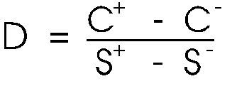 {9}
{9}
In other words,
D in some sense tells us the amount the option changes in value
for a given change in the value of the underlying. (This is not
strictly true. The underlying never goes form S+ to S-, but from
S to S+ or S to S-. However, if we define "change in the
underlying" to mean the difference between one underlying
value and another, this interpretation is valid). It is thus a
measure of sensitivity of the option to changes in the underlying
asset. This is precisely why we want to sell D units of the underlying
to hedge one call option, because that will make each position
equally sensitive to one point moves in the underlying asset.
Why
probability drops out
You might
have noticed that nowhere in our construction of the tree, nor
in working backwards to get option values, did we make any explicit
statement about the probability of an up or down move. While this
seems counterintuitive, it is actually a general result of hedging.
We are claiming
in the binomial model that from any state of the world, there
are only two states that can occur next period. But if we can
create a portfolio that is worth the same amount as the option
in each state, we are indifferent which state is realized. Whether
the probabilities of the states are 99 and 1, or 50-50, we are
still going to replicate the option's payoff. Likewise, the person
who has created a hedge portfolio will have no cash flow next
period, so he really doesn't care which state of the world is
obtained, since his economic worth is the same either way.
Why
not up, down, or unchanged prices?
One criticism
of the binomial model is that it is unrealistic to assume that
the underlying asset can take on only two values over the next
time period. When the time period is a month, that is certainly
true. We will describe shortly the effects of making the time
period extremely small, so that the resulting path of prices is
much richer than what we used above. But as small as the periods
get, it seems much more reasonable to assume that price can up,
down, or stay the same.
This may be
true, but unfortunately, that would leave us with an unsolvable
problem as we've set it up here. The reason is that we would have
three states of the world, and therefore three equations to solve
with only two unknowns. Three equations with two unknowns is,
in general, an unsolvable problem. It was no accident that we
assumed things the way we did. Note, though, that over two periods
the underlying asset does take on three values, one of which is
nearly unchanged (we will fix this one later, too). If we think
of every two model periods as being one real world period, things
don't look as unrealistic as they may have at first.
Shortening
the period
In our example,
we made each period a month in length. If we like, though, we
can make each interval as small as we want. A tree of minute by
minute changes ought to be precise enough for most people. Whoever
is not satisfied with that need merely tell us what period is
short enough so that an up and down move isn't a bad representation
of reality, and we will use a period of that length. If they claim
that the asset can take on five values after one second, then
we will make each period one fourth of a second, which will yield
five values per second.
When we shorten
the period, it's important to change a couple of things when building
our tree of prices. The first is that the risk free rate must
represent the borrowing rate over that interval. If we are working
with days, then .%5 per month translates to about 1.6 basis points
per day. The second is that the size of the up and down moves
must obviously be smaller. But how much smaller?
The answer
to this question depends upon what type of distribution we feel
the underlying asset's price follows. It's beyond the scope of
this paper to discuss different ways to make u and d be a function
of the number of periods, and the types of distributions these
imply. But Appendix B does cover the mathematics of one method
that allows us to have a stable set of option prices as we increase
the number of binomial periods. Jumping straight to the conclusion
presented there, we get:
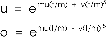 {10}
{10}
| where |
mu |
is the annualized mean of the natural log of the return
on the underlying asset |
|
|
v |
is the annualized standard deviation of the natural log
of the return on the underlying asset |
|
|
t |
is the number of years to expiration of the option |
|
|
m |
is the number of binomial periods |
|
If we pick
u and d according to {10}, then no matter how many periods (m)
we have in our tree, the mean and standard deviation of the underlying
asset in the tree will be mu and v.
How
many periods are enough?
When we use
the binomial model, we are free to break the option's life into
as many periods as we choose. This probably did not concern you
when it seemed as if we could make the period arbitrarily small
in length. But we can also go in the other direction, allowing
the asset to move only up or down over a half-year, a year, or
any other amount of time that evenly divides up the option's life.
It seems intuitive that that will not work very well, and in some
sense the intuition is correct. Even though we have constrained
the total variance of the underlying asset over the term of the
option to be invariant to our choice of periods (See Appendix
B), it turns out that the value of the option the binomial model
gives us is still a function of the number of periods used.
Fortunately,
as we increase the number of periods, the model converges to the
"true" value of the option. An example of this is shown
in Table 1, where a call option is valued using the binomial model
with the number of periods varying from 1 to 150.
| Number of Periods |
Option Value |
| 1 |
7.45 |
| 5 |
6.25 |
| 10 |
5.80 |
| 15 |
6.05 |
| 20 |
5.88 |
| 25 |
6.01 |
| 50 |
5.92 |
| 75 |
5.97 |
| 100 |
5.94 |
| 125 |
5.96 |
| 150 |
5.94 |
Although
it cannot be ascertained from the table, it should be obvious
that as we use more periods, it takes much longer to calculate
option values. We are faced with a tradeoff between speed and
accuracy.
COMPARING
THE EXPECTED VALUE TO THE BINOMIAL
We have now
seen three different way to value an option:
expected value
using the payoff diagram, simulation (also a form of expected
value) and the binomial. In this section we'll compare the prices
these three models yield, and demonstrate mathematically why the
binomial is also a form of expected value model.
Turning
our two equations into a simpler formula
In Section
2, we set up a portfolio that replicated a call option by holding
D units of the underlying, and borrowing B dollars. When we solved
for these two values, we plugged in actual numbers. It is a bit
simpler, though, to solve for them more explicitly. Notice that
our equations are always:
D (S u) -
B (1=r) = C+
D (S d) -
B (1+r) =C-
D S - B =
C {11}
We are going
back to our original definition of u and d as the rate of return
on the underlying. Simple rearrangement of these two, shown in
Appendix A, yields:
 {12}
{12}
Let's call
 {13}
{13}
so that
 {14}
{14}
Note that,
by our dominance argument, both p and 1 - p must lie between zero
and one. This means that p (and 1 - p) can be thought of as probabilities.
Not that they are true probabilities, of course, but they can
be thought of that way.
If we do,
then what we end up with is that the value of the call is equal
to the expected value of the call next period, discounted back
over one period at the risk free rate. The weights that we use
in our averaging are the pseudo-probabilities in the above formula.
By applying this reasoning throughout the tree (since it holds
in every node), we show in the next section that the value of
the call today is equal to the discounted expected value of the
call at expiration, where the probability function we use is a
binomial with the probability of up move equal to p.
It bears repeating
that we are not saying here that the probability of an up move
is this amount, just that if we pretend that it is, we can solve
for the call value directly.
All of which
means that the discounted expected value formula described in
the first section has a lot more power than at first appeared.
Generalizing
the Result
Our above
equation states
 {15}
{15}
If this is
true in each node just before the option expires, we are saying
that the value in that node is the weighted average of the two
intrinsic values coming out of that node, discounted one period.
But if we go back one more period, the same statement can be made:
that the value in any node in the third to last period is the
discounted weighted average of the option values in the second
to last period coming out of that node. But if each of these is
a weighted average of the intrinsic value, we can substitute back,
and say:
 {16}
{16}
where
|
C++ |
is the intrinsic value after two up moves |
|
|
C+- |
is the intrinsic value after one up move and one down move
|
|
|
C-- |
is the intrinsic value after two down moves |
|
These three
states are the only possibilities when we are sitting in the third
to last period. We thus can make the option value in each node
in the third to last period a weighted average of only the intrinsic
values of the three nodes that can be reached from that node in
the last period (it's a weighted average because p2 is the probability
of going up twice, (1-p)2 is the probability of going down twice,
and 2 p(1 - p) is the probability of either going up and then
down, or down and then up). This is crucial, because we can also
do this for the fourth to last period, making all the option values
in that period weighted averages of the intrinsic values those
nodes can reach in the last period. Carrying this all the way
back to the base of the tree, the value today is a weighted average
of all the values the option can also do this for the fourth to
last period weighted averages of the intrinsic values those nodes
can reach. Carrying this all the way back to the base of the tree,
the value today is a weighted average of all the values the option
can have in the last period. Thus we can say that:
an option's
value is simply its discounted expected intrinsic value.
Successively
back substituting as above, the exact formula for the option value
today as a function of the values it can hit in the last period
is:
call=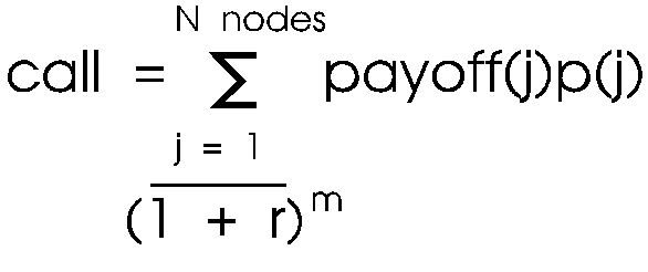 {17}
{17}
where payoff
| (j) |
is the option's intrinsic value with j up moves |
|
|
| p(j) |
is the pseudo-probability of reaching node j |
|
|
| m |
is the number of periods to expiration |
|
|
The pseudo-probability
comes from the binomial distribution, and with N nodes, the probability
of the underlying finishing in node j is:
 {18}
{18}
Equation (17)
looks a lot like (3), when (3) is adjusted for discounting. As
we said before, the technique used to get (3), counting boxes,
is similar to integration. Equation(17) is an integration technique,
as well. In both cases, they are numerical approximations; the
more points one includes in the formula, the more exact the answer
will be. By using the analytical tools of calculus, one can also
obtain the exact solution to the problem, where there are an infinite
number of points used. This is the famous Black-Scholes formula:
 {19}
{19}
where
| S |
is the price of the underlying |
|
|
| X |
is the strike price |
|
|
| r |
is the continuously compounded interest rate |
|
|
| t |
is the number of years to expiration |
|
|
| N(d1) |
is the area under a normal curve to the left of d1 |
|
|
| v |
is the annualized standard deviation of the log return on
the underlying |
|
|
|
|
|
|
and
 {20}
{20}
This formula
yields a value which will agree with the binomial, when the binomial
is run with an infinite number of periods. Short of that, the
binomial will converge to the Black-Scholes value as the number
of periods is increased. Before we leave the binomial, it is interesting
to look at the expected rate of return on the underlying asset,
using the pseudo-probability just derived. We know that the expected
value of S next period is
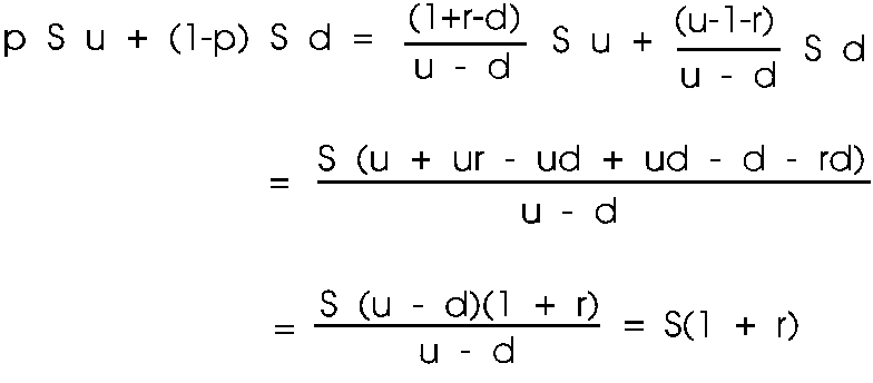 {21}
{21}
This means
that the expected return on the underlying is equal to the risk
free rate. The implication to this is that investors are risk
neutral, so that regardless of the risk of an asset, they only
need to get the same rate of return as they could get from a riskless
investment. Again, this doesn't mean investors really are risk
neutral, just that the pseudo-probability implies it.
Comparing
option values from the different pricing models
Table
2: Comparison of Simulated Option Prices to the Binomial
| Model |
Strike |
|
100 |
110 |
120 |
| Lognormal |
11.28 |
5.91 |
2.69 |
| Contaminated lognormal |
11.96 |
6.34 |
2.93 |
| Normal |
11.52 |
5.93 |
2.47 |
| Contaminated normal |
11.39 |
5.96 |
2.70 |
| Binomial |
11.29 |
6.01 |
2.68 |
| Black-Scholes |
11.31 |
5.95 |
2.71 |
| Historical |
17.47 |
13.36 |
9.68 |
| Binomial |
18.4 |
14.22 |
10.50 |
Table 2 presents
the values of some options that were calculated using the binomial,
as well as from some of the types of simulations discussed above.
In each case, the option is a one year European call, with the
underlying asset trading at 100. The risk free rate used was 19%
per year. Three different strikes were used, one each for in,
at, and out of the money options (the 110 strike is much like
an at the money option, in that this is the expected price of
the underlying at expiration, using the pseudo-probabilities as
above). Simulations were run assuming simple normal and lognormal
processes, as well as contaminated versions of each. The contaminated
returns were generated in such a way that they had an ex-post
variance that was the same as the variance of the uncontaminated
returns. In addition, a bootstrap simulation was run, using gold
prices from January '78 to October '86, and assuming a multiplicative
process. The binomial values below the gold option prices are
derived using the realized standard deviation form the simulated
gold returns.
The comparison
of the pricing models appears in Table 2. Each column represents
a different strike price. The first two lines are simulation results
obtained by assuming the underlying asset follows a lognormal
random walk. Of the two, the first line is for a walk with a stationary
standard deviation of 15%. The next line is the contaminated distribution.
For this, a random variable was drawn to determine the volatility
for each return period, so that over time the variability jumped
around. For each strike, the option value from the contaminated
distribution is higher than the simple lognormal. This is because
the asset with the contaminated return process has a higher probability
of both very low returns and very high returns compared to the
simple lognormal. Since the value of an option comes from the
chance of very high returns with limited loss on the downside,
this is a perfectly reasonable result. Given the number of simulations
run and the variance of the underlying asset, each value has a
confidence interval of roughly .1.
The next two
lines contain similar data, for a normal distribution instead
of a lognormal. The contaminated distributions yield higher option
values, but only in two out of three of the strikes, and not by
as much.
On the fifth
line the price of an option valued using the binomial algorithm
is shown. For all three strikes, the price is very close to the
straight lognormal. This is because the binomial was shown earlier
to be a weighted average formula, where the process generating
the weights converges in the long run to a lognormal distribution.
Below the binomial, the exact price of the option, from Black-Scholes,
is shown. Interestingly enough, the contaminated normal option
values appear to be very close to Black-Scholes, just about as
close as the straight lognormal and the binomial model. But we
know this must be a byproduct of the particular contamination
method used, since the straight normal is a special case of a
contaminated normal, and it does not perform nearly as well as
the others.
The results
of running simulations for gold options is presented in the lower
portion of Table 2. In each case, the binomial value is consistently
higher than the simulated value. The frequency distribution of
the simulated gold returns is presented in Figure 8. The x axis
is the ending value of $1 invested in gold, the y axis is the
ending value of simulations (out of 2000 again) that realized
that return.
Figure
8. Frequency of Simulated Gold Returns
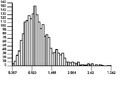
The graph
itself appears to be a cross between a normal and a lognormal,
in that it is symmetric in the center like a normal, but has a
much bigger tail on the right and not much on the left, like a
lognormal. This partially explains the large difference between
the historical and binomial values.
CONCLUSIONS
This paper
has derived three related methods for valuing simple options:
the discounted expected value method using a probability function,
the binomial model, and simulation. It has shown that the three
in theory amount to the same thing, and has presented results
that bear this out.
APPENDIX
A
DERIVING
THE DIRECT FORMULA FOR THE OPTION IN EACH NODE
The two equations
which state that the value of our portfolio must be the same as
the value of the option, in the next period m are
D(S+) - B(1
+ R) = C+
D(S-) - B(1
+ R) = C- {A.1}
We can subtract
the second equation form the first, as we did before, to get {9}.
Given that:
S+ = Su, and
S- = Sd, we
have
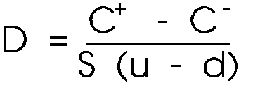 {A.2}
{A.2}
Substituting
back into the first,
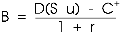 {A.3}
{A.3}
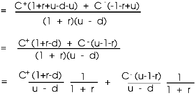
Given D and
B, the value of the call is given by
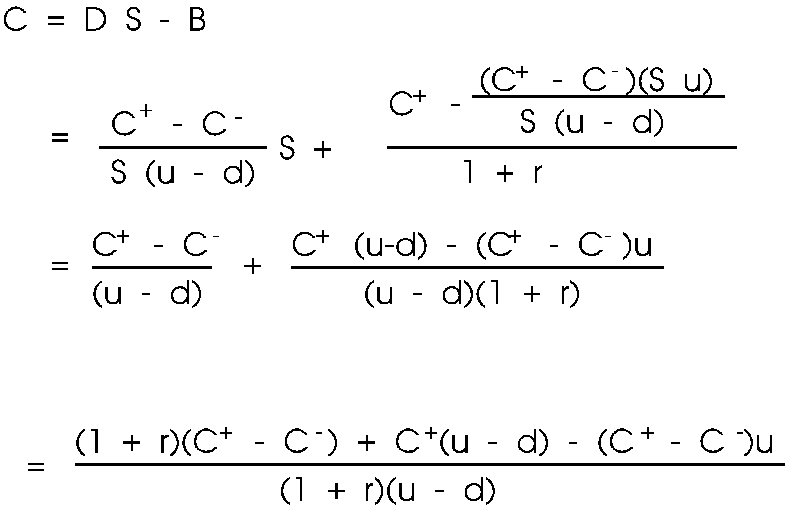 {A.4}
{A.4}
 {A.5}
{A.5}
APPENDIX
B
HOW
TO CHANGE u AND d FOR DIFFERENT NUMBERS OF BINOMIAL PERIODS
If
we know what values of u and d we'd like to use to price the option
for a given number of binomial periods, how do we adjust them
when we want to use more periods? That is the question addressed
here. We begin by outlining the procedure.
We
first assert that the variance of the underlying asset's price
at expiration implied by our tree should be independent of the
number of periods used. We get a formula for u1 and d1 in terms
of u and d, where u and d were picked for a given number of periods
(call it n), and u1 and d1 are the jumps when we have a different
number of periods (some multiple m times n). Thus, it should come
as no surprise that u1 and d1 are functions of u, d, and m.
We
then state that the mean of the underlying asset's price at expiration
should be the same no matter now many binomial periods we use.
This gives us another relationship for getting u1 and d1 as a
function of u, d, and m.
Putting both
of these together, we derive a unique way to choose u1 and d1.
By assuming a special form for u and d, we are then able to make
the transformation for more periods a very simple transformation.
The remainder of the appendix lays this out in greater detail.
One thing
we know is that the probability distribution of the underlying
asset's value at the option's expiration had better be independent
of how we are breaking up time. If the uncertainty of the underlying
price in three months is such that we feel it will have a return
that is between -5% and 10% with probability one-half, that range
and probability should be implied by our jump sizes and probabilities,
regardless of the period length. Now, let us suppose that no matter
what length of time we choose one period to mean, the probability
of an up move (down move) is the same. In other words, if there
is a .7 chance of an up move when each period is a month, then
there is also a .7 chance of an up move over one minute. (Although
we said before we didn't need to know the probabilities of each
move to value the option, they will be useful here to help us
build the tree based on the asset's mean and variance. If we instead
somehow know exactly what the up and down moves are, we don't
need to calculate them, and have no need to know the probabilities.)
Let's use these two statements to determine how to adjust the
size of our moves when we change the length of a period.
If the price
of the underlying is S right now, then after an up move it will
be S u. After another up move, it will be S u2. Over n periods,
there will be n moves, so if there are j up moves, there are n-j
down moves. This allows us to say that after n periods, the price
should be S * u^j * d^(n-j),where j is the number of up moves
experienced. If we call this price S*, then we have
 {B.1}
{B.1}
To make things
computationally simpler, let's deal with the natural logs of u
and d when referring to up and down moves, ln(u) and ln(d). This
will allow us to add and subtract instead of multiply and divide.
Now, taking the log of both sides, we have
ln(S*/S) =
j ln(u) + (n-j) ln(d) = [ln(u) - ln (d)] + n ln(d) {B.2}
This quantity
represents the log of the rate of return on the underlying asset.
We can get the variance of it by taking the variance of the terms
on the right hand side. The random variable here is j, the number
of up moves. Since the variance of a constant is zero, and the
variance of a random variable times a constant is the square of
the constant times the variance of the random variable by itself
(var(Cr) = C2 var(r)), we get
Var(lnS*/S)
= Var(j) [ln(u)-ln(d)]²
= ln(u/d)²
Var(j) {B.3}
We now have
a measure of the variance of the asset's return over the option's
life, as a function of the up and down moves that can be experienced
over one time period. Since j is a variable that is binomially
distributed (the name of the model had to get into this somewhere),
it has a variance of np(1-p), where p is the probability of an
up move. What we'd like, then, to be sure the total variance is
independent of the length of our periods, is to have
Variance over
n periods = Variance over 2n periods = Variance over any number
of periods
Let's use
n and mv to solve our problem of adjusting u and d for the length
of a period. We have
ln(u/d)²
Var(j) = ln(u1/d1)² Var(k) {B.4}
where
| j |
represents the number of up moves in a tree with n periods |
|
|
| k |
represents the number of up moves in a tree with mn period |
|
|
All we've
done here is say that if we have m times as many periods, then
an up move is going to be u1, and a down move will be represented
by d1. Ultimately, the question to be answered is: 'What is u1
as a function of u, and d1 as a function of d?' Just as j was
the number of up moves with n periods, k is the number with mn
periods. But recall that k, too, must be binomially distributed,
so its variance will be (mn)p(1-p). We can do this because we
assumed that the probability of an up move was independent of
the period size. So Var(k) is just m time the Var(j). We then
get
Dividing both
sides by Var (j),
ln(u/d)²
= m ln(u1/d1)² m {B.5}
therefore
 {B.6}
{B.6}
What this
tells us is that, given u and d, if we multiply the number of
periods by m, then u1 and d1 must conform to {B.6}. There are
infinitely many pairs of u1 and d1 that will satisfy this, because
{B.6} is only one equation, with two unknowns. But another constraint
to add to this is that the mean, too, be independent of how many
binomial distribution, the mean after n periods is equal to n
times the mean after one period. If we call the mean of the log
return over the life of the option LM, we have
n[p ln(u)
+ (1 - p) ln(d)] = LM
m n [p ln(u1)
+ (1 - p) ln(d1)] = LM {B.7}
since the
one period log mean is the weighted average of the log of the
up and down moves, and again the lifetime mean should not depend
on how many periods we are using.
Thus
 {B.8}
{B.8}
 {B.9}
{B.9}
Using {B.6}
in the denominator,
 {B.10}
We now have
a way of going from u and d to d1 (and therefore u1, using {b.6})
and we increase the number of binomial periods by a factor m.
With u and d for, say, 1 binomial period, if we want to increase
the number of periods to 10, we use u, d and 10 in {B.10} to get
the ln of d1, and use this in {B.6} to get the ln of u1.
To make this
look simpler, let's suppose that
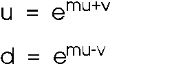 {B.11}
Here, mu is
the mean log return over one period, and v is the amount the log
of the return exceeds the log of the mean in an up state, or falls
below the log of the mean in a down state. Substituting {B.11}
into {B.10}:
 {B.12}
For the special
case where p = .5, this reduces to
 {B.13}
After all
that, this says that if we want to double the number of periods,
then we cut the mean in half, and divide v by the square root
of 2. Since many people like to thing in terms of annualized means,
let mu and v denote the values we'd pick if each binomial period
were a year in length. Then we can apply {B.13} with m representing
the number of binomial periods in a year.
Let's look
at some properties of the distribution given this method for building
the tree. If mu and v are set for a period length of a year, we
have
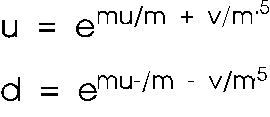 {B.14}
where m represents
the number of binomial periods per year.
Defining u
and d according to {B.14}, with p = .5, the mean of the log return
over one period is
 {B.15}
as expected.
But we can also calculate the variance:
 {B.16}
Since the
variance over one period is v2/m,. the variance is v2 over m periods
(one year). (This assumes that the process is normal. Since we
are dealing with logs, we are making the log of the process normal,
and the return process itself is lognormal.) We now know how to
pick v; it is the annual standard deviation, and m the number
of periods per year.
One property
that is particularly appealing about this can be seen if mu is
set equal to the risk free rate. In this case, u will always give
the asset a return greater than the risk free rate, and d below
it. Recall that one assumption will be met, no matter what m we
use.
