Advanced
Option Pricing
by
Rich Tanenbaum
(from Topics
in Money and Securities Markets, Bankers Trust Company, Money
Market Center, May 1989.)
INTRODUCTION
In an earlier
paper, "Basic Option Pricing," Topics in Money and
Securities Markets,July 1987, several methods for valuating
options were presented. Chief among these was the binomial model.
Its usefulness, as described in the earlier paper, was limited,
in that the option was assumed to be a European call on a non-dividend
paying stock. This paper will partially complete the analysis,
providing extensions to the binomial to handle puts, American
options, cash flows on the underlying asset, and options on assets
other than stocks, as well as relax some of the assumptions made
there.
AN EPIDEMIC
OF EXTENSIONS
Valuing
Puts with the Binomial
As a way of
reviewing the binomial, let's present how to price European put
options. with it. We are again assuming that
- the underlying
asset can go only up or down over a discrete period
- these jumps
are known, and constant in size
- the risk
free rate is known and constant
- we can
borrow or lend at this rate
- there are
no taxes or transaction costs
- we can
buy and short the underlying asset, in any amounts
- the underlying
asset pays no dividends over the life of the option
Given the
price of the underlying today, as well as the jumps that may be
achieved, we can draw a tree of all the possible values the asset
can take on from today until expiration. Such a tree is shown
in Figure 1, where the underlying is worth 100 today.
Figure
1: Possible Price Paths Over 2 Periods of an Asset Priced at 100
Today
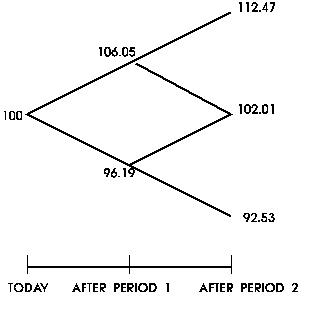
Our goal is
to price the option in the base node of the tree, today. While
we cannot do that directly, we can simply determine the value
of the option in the three nodes, or states of the world, that
can exist at expiration. In this case, since we are valuing a
put, the intrinsic value of the option at expiration is equal
to
max(0,strike
price - underlying price) {1}
We will fill
in the values of the put with 100 strike in each of the three
nodes, based upon {1}, and have Figure 2.
Figure
2: Possible Values of a 100 Put After Two Periods, with Associated
Underlying Asset Prices
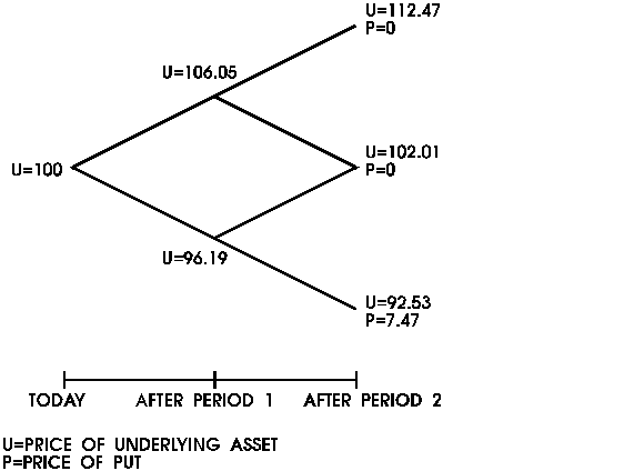
Now let's
look in the node where the underlying is worth 96.19 (one period
from now). The put can have two values after that, 0 and 7.47.
What we are going to do is construct a portfolio in that node,
with underlying at 96.19 and borrowing and lending allowed at
1% per period, that will be worth 0 if the underlying goes up,
and 7.47 if the underlying goes down. This portfolio will have
D shares of the underlying, and lend B dollars. To calculate D
and B, we must solve:
102.01 + B
(1+.01) = 0 {2a}
92.53 D +
B (1+.01) = 7.47 {2b}
This says
that the portfolio value after an up move (the left hand side
of {2a}) must equal the put value after an up move (the right
hand side of {2b}, and the portfolio value after a down move must
equal the put value after a down move.
With two equations,
and two unknowns (D and B) we can solve {2}quite easily. The value
of this portfolio of D and B is always going to be worth the same
as the option in that node, as well. This value
96.19 D +
B {3}
is the value
of the option when the underlying is worth 96.19.
We can apply
this reasoning to get an option value in all the nodes in the
second to last period (see Figure 3).
Figure
3: Underlying Asset, Replicating Portfolio and Option Values

But knowing
those put values allows us to create a portfolio in each node
in the preceding period that will replicate the option, and therefore
have the same value in those nodes, as well. We can use this all
the way back to the base of the tree, and say the value of the
replicating portfolio using today's prices is the value of the
put option.
Given all
that, what was the difference between the way we priced puts and
calls? Only the formula we use to get the intrinsic value of the
relevant option in the last period of the tree. For the put, we
used
max(0,strike
price - underlying price) {1}
whereas a
call would have used
max(0,underlying
price - strike price) {4}
Combination
positions
We can extend
this reasoning to make the pricing model even more flexible. Suppose
we want to value a portfolio of two call options with the same
expiration, but different strikes. Rather than use our binomial
model twice and add the answers together, we can save ourselves
some time and effort by building one tree of underlying values,
and then at expiration calculate the intrinsic value of the combined
position. We then work out what portfolio would replicate the
total cash flows. The portfolio value today that replicates the
flows must be worth the same amount as the portfolio of two options.
Following
this reasoning, we can also include puts (via {1}) as well as
positions in borrowing or lending, or positions in the underlying
asset, as part of the portfolio we are trying to replicate. If
we include borrowing and lending of $x today, the tree will contain
the future value of x in each node at expiration. If we are replicating
the underlying asset, it is worth the value of the underlying
asset in that node, of course.
For example,
if we had a position that was long a 110 call, long a 95 put,
long the underlying and long 50 par amount of a bill maturing
at the options' expiration, then a table of intrinsic values of
this position can be obtained (shown in Table 1).
Table
1: Valuing a Portfolio at Expiration
| Underlying at Expiration |
Call |
Put |
Underlying |
Bill |
Total |
| 85 |
0 |
10 |
85 |
50 |
145 |
| 90 |
0 |
5 |
90 |
50 |
145 |
| 95 |
0 |
0 |
95 |
50 |
145 |
| 100 |
0 |
0 |
100 |
50 |
150 |
| 105 |
0 |
0 |
105 |
50 |
155 |
| 110 |
0 |
0 |
110 |
50 |
160 |
| 115 |
5 |
0 |
115 |
50 |
170 |
| 120 |
10 |
0 |
120 |
50 |
180 |
By extending
this table, and making the increments finer, we could value the
whole portfolio in each node at expiration once and only once,
and then work out what portfolio today would replicate that value
at expiration.
Put-call
Parity
One thing
to notice about valuing puts and calls is that whichever equation
is used, {1} or {4}, the intrinsic value of the option is never
negative. We knew this already, that an option will never be exercised
if it is out of the money. Since we have shown in an earlier paper
that the binomial ends up giving us a weighted average of the
intrinsic values, we can see that the option values it returns,
weighted averages of all non-negative numbers, will conform to
rational economic theory.
We can look
at {1} and {4} another way, too, to derive an important relationship
between put and call prices, named "put-call parity."
Imagine all
the nodes the binomial tree generates at the expiration of the
option. For a given strike price, in each node the underlying
price is either above, at, or below the strike. This means that
in each node, either {1} or {4}, but not both, is positive. In
one special case, where the underlying in a node is equal to the
strike, they'll both be zero. Now suppose you have a long position
an a call, and a short position in a put, both with the same strike.
The value of your total position at expiration in the nodes that
are above the strike is
underlying
asset - strike
and in the
nodes below the strike is also
underlying
asset - strike.
This is true
no matter what the strike is, as long as it's the same for both
the put and the call. Let's suppose you also buy a bill maturing
at the expiration of the option, which will have a maturity value
of the strike price. Combined with the put and call, the value
of this position will be exactly equal to the underlying asset
at expiration. Finally, if you short sell the underlying asset
today, then at expiration your value will net out to zero. So
a portfolio of
long call
+ short put + short underlying + lend present value of strike
will be worth
zero in every state of the world at expiration. Therefore, it
should not have any value today to avoid arbitrage. Thus, put-call
parity states that
put = call
- underlying + present value of strike{5}
If you want
to use the call valuation model, applying {5} will generate a
put value (as long as all the above assumptions are met, particularly
the fact that we are valuing European options).
Options
of Futures
In valuing
options on futures, we need to adjust our algorithm slightly,
but the changes are surprisingly minor. First, the stock price
had to have up and down moves which surround the risk free rate
to avoid dominance. However, a futures contract doesn't require
money be put up that could be earning money elsewhere. Therefore,
the up and down moves on a futures contract ought to surround
a zero rate of return (we may have to put up margin, but since
we can keep the interest the margin earns, we don't lose the use
of the money). With a multiplicative process, as we have used
before, this would lead, for example, a futures currently prices
at 50 to rise to 50 x 1.02 or fall to 50/1.02.
The next change
is in the two equations and two unknowns. We still want to make
the value of the replicating portfolio be the same as the value
of the option in each node, but owning a futures contract causes
a marking-to-market profit/loss, and also the futures position
itself has no value. Thus, holding D units of a contract, and
lending B dollars, our new equations become:
D (F+ -F)
+ B (1 + R) = C+
D (F- -F)
+ B (1 + R) = C- {6}
where
| F |
is the futures price in this node |
| F+ |
is the futures price after an up move |
| F- |
is the futures after a down move |
| R |
is the one period interest rate |
| C+ |
is the option price after an up move |
| C- |
is the option price after a down move |
Since the
futures doesn't cost anything to hold, our final adjustment is
to note the value of the replicating portfolio is just B.
Even with
these changes, the value of D is still
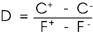 {7}
{7}
which makes
sense, as this is the same form as the formula for the derivative
of C with respect to F, the basis for hedging (the derivative
is taken over a change in the underlying, one binomial period
hence. As the number of periods increases, this approaches the
instantaneous derivative).
The formula
for B, and thus the option value, is
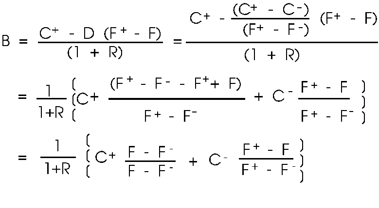 {8}
{8}
Just as in
the binomial model on an asset, the option value in a node is
the present value of the up and down option values that can be
reached from that node, weighted by pseudo-probabilities (numbers
which sum to one, and are both between 0 and 1).
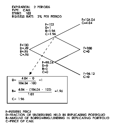
Figure 4 presents
a simple tree that demonstrates the pricing of a call option on
a futures contract.
Figure
4: An Option on Futures Example
Options
on Forwards
In an efficient
market, without stochastic interest rates, a forward and future
on the same commodity with the same delivery date should be priced
the same. (Although the futures will have intermediate cash flows
due to marking-to-market, that can be hedged by holding, with
T years to delivery and a rate r to delivery, 1/(1+r){to the T
power} futures contracts for every forward to be hedged. This
strategy will lead to the same position value at delivery as holding
one forward contract.) Therefore, to value an option on a forward,
we start by building the tree of underlying values exactly the
same as we do for a futures option, as above. The only difference
is that, in the next step, our two equations in two unknowns must
take into account that, in current dollars, the profit/loss from
the forward must be discounted back from delivery to the node
in which we are solving the equations:
 {9}
{9}
where T is
the time from the period after the underlying has moved to the
delivery of the forward contract.
As with futures,
the cost of the replicating portfolio is B, since the forward
contracts held have no value today. This time, D will be:
 {10}
{10}
which again
is perfectly reasonable from a hedging standpoint, since the profit
on the forward itself must be discounted to the present. The formula
for B, interestingly enough, reduces to:
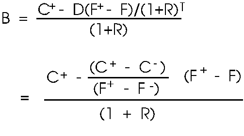 {11}
{11}
which is the
same as the value of the option on a futures contract. This is
sensible; since all the F's are the same, and the intrinsic values
at expiration are the same, then the C+'s and C-'s are all the
same.
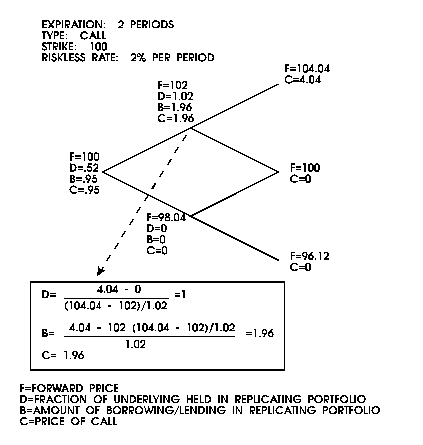
In Figure
5,. a tree to value a call option on a forward is shown.
Figure
5: An Option on Forward Example
American
Options
So far, all
the options have been European. To turn any of them into American
options models, we need only recognize one very simple rule: an
American option can never trade for less than intrinsic value.
If, during our walk backwards through the tree, we come up with
a replicating portfolio that is worth less than intrinsic value,
we substitute intrinsic value for the option in that node, and
know that the option will be exercised at that point.
This may seem
somewhat simplistic and arbitrary. After all, the replicating
portfolio is supposed to yield portfolio values to match the option,
so why should we adjust afterwards? The reason is that the construction
of the replicating portfolio assumes the option will exist in
the next period. But any time the intrinsic value of the option
is more than this amount, the option holder is looking at holding
an instrument whose value next period can be replicated more cheaply
by holding other assets. Holding the option seems useless. He
could try selling the option, but no one will pay more than intrinsic
value (since next period they will be left with something worth
less than the intrinsic value today), so the only way out of the
dilemma is to exercise the option immediately. At this point,
if he were to sell, instead, he would be indifferent between exercising
or selling at intrinsic value.
To recap,
as we work through the tree, after solving for the cost of the
replicating portfolio, we make the option value OV
OV = max(replicating
portfolio value, intrinsic value) {12}
Looking at
this from another angle, we can also see the obvious rule for
exercising an option early; only exercise when the option is trading
at the intrinsic value. If it has any time premium (the
excess over intrinsic value) you could realize more by selling
the option.
A classic
example of this is the proof that it is never advantageous to
exercise an American call on a non-dividend paying stock early.
Suppose you are long a call option with strike price K. The underlying
is worth S now, and is in the money. If you exercise now by borrowing
the strike at rate R to expiration you will have the underlying
less K x (1 + R) with certainty. On the other hand, if you wait
until expiration, you will have the underlying less K if the call
is in the money, and 0 otherwise. Either way, you are ahead by
waiting until the last minute to exercise your call.
One thing
that we lose with American options is the ability to use the simple
expected value formula to price the option. Now, not all the nodes
of the tree will be reached, if there's a possibility of early
exercise. The expectation must then use a complicated conditional
distribution.
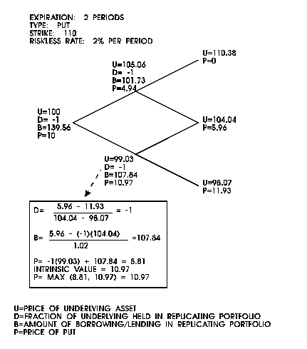
Figure 6 gives
an example of pricing an American put option.
Figure
6: An American Option Example
Cashflows
on the Underlying Asset
Another major
restriction we've imposed so far is that there be no cashflows
on the underlying asset. This leaves out dividend paying stocks
and even spot foreign exchange. (It does not leave out most options
on debt instruments, even those with coupons. These are "cash
flow protected" in that the strike price at a given time
reflects the accrued interest on the exercise date, which means
the amount that must be paid to exercise a call before a coupon
date is more (by the amount of the coupon) than what it costs
to exercise the call right after a coupon is paid.) We will now
remedy that.
In the absence
of taxes, if the only uncertainty concerns the price of the underlying
asset next period, an instrument's total return over a day ought
to be the same whether a cashflow was paid or not:
 {13}
{13}
This means
that if the cashflow is 2% one day, then the price should drop
by 2% to reflect that (net of other factors). For a stock, the
firm has lost value by an amount equal to the cash distribution.
To keep the
same return process as we've already used for the binomial, what
we will do instead is, in those periods when a cash flow is to
be made, make the up price be:
S+ = S x u
- cash flow+ {14}
and the down
price
S- = S x d
- cash flow-
where
S is the price
in the node before the jump
u is the size
of the up jump for an equivalent, non-cash paying asset
d is the size
of the down jump for an equivalent, non-cash paying asset
This assumes
we know what the cash flow will be, and when. For stocks, this
will most likely mean choosing periods closest to quarter year
intervals (when dividends are paid), to use the special form of
{14}. For foreign exchange, where the option is on spot currency,
we might assume that it is earning a daily coupon equal to the
short term rate in that currency.
In making
a statement about the size of the cash payment, we can calculate
it in a variety of ways. We can have a forecast of dividends in
dollars, for instance the dividend stream can be 2, 2.2, and 2.42
over the option's life. We can also be a little fancier, and make
the dividend be a percentage of the asset's price in each node.
This would lead to higher dividends for higher stock prices. In
fact, we can have any type of function of the stock price we want,
so long as it is a function of just the stock price and the time
period, and not other factors we have not included in our model.
Note that if we are going to pick certain arbitrary dividend patterns,
we may have to use the bushy tree version of the binomial, described
in the section on non-constant volatility.
Armed with
a new way of building the tree, we will continue to calculate
the option value by looking at the intrinsic value at expiration
(using these new, cash flow affected prices of the underlying
in the tree). Our two equations in two unknowns will recognize
that holding a portion of the underlying may give us a cash flow,
as well:
 {15}
{15}
where CFi
+ (CFi-) is the cash flow in the ith binomial period, after an
upmove (downmove). We have CFi here, unlike before, but since
it is known we can still solve for D and B as easily as before.
Once again, the option value is the value of the replicating portfolio,
D x S+B.
Figure 7 shows
an example of valuing a call option on spot FX, which assumes
a cash flow each period.
Figure
7: An FX Option Example

European/American
Options
Some options
are hybrids of American and European. They are exercisable on
certain dates, but not on others. The prime example of this is
the call option embedded in many bonds. They are not callable
for the first few years after issue, but after that they may be
exercised any time up to maturity. These are very simple to handle
with the binomial. Merely invoke {12} only in those periods after
the first call date: if the option is American in that period,
make sure it is worth at least intrinsic value. If it is European
in that period, the option is worth the value of the replicating
portfolio.
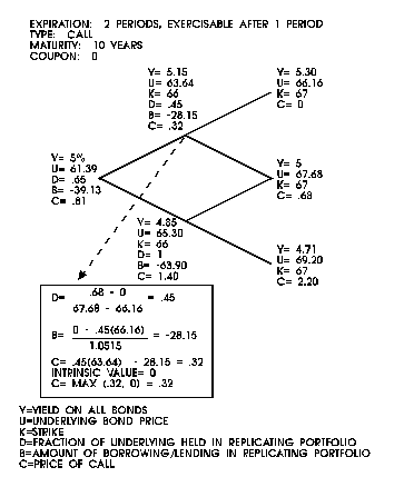
In Figure
8, a bond call option example is shown, with a changing strike,
that is not exercisable in the first period.
Figure
8: A Hybrid American Bond Option Example with Changing Strike
Options
on Bonds
In an earlier
paper, we introduced a way to value options on bonds using the
binomial model (see "Assessing the Value of a Callable Eurobond,"
Topics in Money and Securities Markets, July 1987). We
will quickly restate the idea here. First, we want to point out
why it is important to cast the model the way we do.
When we apply
the binomial to a stock, we first place the current price in the
base node. We then apply the up and down moves to this price.
As we go further out, we continually apply the same up and down
moves. By the end of the tree, the price is widely dispersed around
the current forward price of the stock. There are two reasons
why this will not work well for bonds. First, as the bond approaches
maturity, its duration declines, and with it its price volatility.
Second, the bond's price must move towards par as it approaches
maturity, whereas the stock price is unconstrained.
The simplest
way around both these problems is to make the bond's yield be
the stochastic variable in the model (the thing that moves up
and down in the tree). If the yield on the bond today is 8%, we
can posit it to go up to 8 x 1.05, or down to 8/1.05. We will
then build the tree using this same 1.05 factor all the way through.
When we are done, we'll have a tree of yields, but using the price-yield
relationship we uniquely convert this to a tree of prices. The
prices will have the property that they will all be converging
to par, and the jumps in prices will be getting smaller as we
move through the tree.
This is fine
as an approximation, but it will turn out that this model has
a number of flaws in it which are quite subtle and difficult to
handle. Nevertheless, the prices that come out will still be fairly
close to those gotten via a more sophisticated and correct model.
It is beyond the scope of this paper to present an algorithm which
addresses these other problems.
Figure 8 is
an example of how to value a call option on a bond when the yield
curve is assumed to be flat, and only moves in parallel. In it,
the option is American after the first period, and the strike
is assumed to change (see the next section).
Options
With a Changing Strike
Certain options
have their strike prices changing over their life. For an example
of this, we can again turn to bonds. If the strike is quoted as
the price such that the bond will yield 8%, then any bond with
a coupon other than 8% is going to have a different strike price
depending on when the option is exercised (this is sensible only
if we are talking about American options). To handle this, we
merely calculate the intrinsic value based upon the relevant strike
before invoking {12}.
This is just
an extension of the way we handled combination positions with
one tree earlier Then, we valued two calls with different strikes
at once. In general, we could have a complicated payoff diagram,
and use the payoff at a given level of the underlying to determine
the intrinsic value. In other words we have a function called
intrinsic value, which is a function of the underlying price at
expiration. IV(S) is a function of S, the underlying asset price.
For a position that is long a 100 call and a 105 call,
IV(S) = max(O,S
- 100) + max(O,S - 105) {16}
Now we are
extending this idea to periods before expiration. We have IV(S,t)
instead of merely IV(S). For a bond with a strike yield of 9%,
if S is the yield in a given node of the tree, we might have:
IV(S,t) =
max (O, price of bond with yield S and t years to maturity-price
of a bond with yield 9% and t years to maturity). {17}
where t is
the maturity of the bond in the binomial period for which the
intrinsic value is being calculated. We don't want to extend the
analogy too far, though. While it is possible to value many European
options with the same expiration with a single pass through the
tree by combining the positions, this is not something we can
really take advantage of for American options. Now, while we can
walk through the tree once, we must keep track of each option's
value individually, which means we won't save very much time.
Figure 8 shows
an example of a call option on a bond with a yield strike.
Including
Taxes
So far we
have assumed there is no such thing as taxes. Unfortunately, that's
not the case. Including them in a pricing model opens a Pandora's
box, which is the second most important reason we don't like them.
Taxes make
our replication path dependent. This term means that
the value of the hedge portfolio at expiration is a function of
how the underlying got there, and not just where the asset ends
up. The path dependence is a result of paying taxes on realized
gains, and not paper profits. For instance, if the underlying
goes up, the delta on a call will rise, and we will buy more of
the underlying asset. Afterwards, when it falls, we sell the underlying
and pay taxes based upon the price or prices at which we initially
bought. Instead, if the underlying falls, we will sell after only
one period and pay taxes at that time (or, to complicate matters
more, we may not have to pay taxes for another year, which means
it's the present value of the tax that we pay). After that, when
the underlying rises, we will be buying, and not pay taxes at
that point. So while the underlying asset has the same value whether
we go up down or down up, the tax payments are different in each
path.
Taxes can
also be different on different types of transactions. While we
no longer have preferential tax treatment for capital gains in
the U.S., that is not true worldwide. And it may not hold forever,
here, either. We need to know the tax status of the individual
or institution trading the option. We need to know whether they
have other income to offset losses incurred in the option or the
hedge portfolio. If they apply existing positions to either side
of the hedge transaction it may be an old trade eligible for long
term capital gains. Futures may be taxed differently form stocks,
which may be different from interest, which may depend on whether
the borrowing or lending was done on an original issue discount
basis. Taxes vary from state to state, and for an option the tax
liability may depend on what type of business the user is in.
In short, it is going to be difficult, if not impossible, to incorporate
all this into a pricing model.
So let's simplify.
Assume all gains are taxed at the same rate, and all losses are
deductible against other gains. Assume also that all taxes are
payable immediately (including tax on other income, so losses
are deductible immediately). We will see that taxes drop out of
the binomial model completely. The intuition for this is that
the option holder is taxed the same as the replicator, so the
amount of money the replicator needs at expiration is the same
on a pre-tax basis as before. We will now present a more rigorous
proof of this.
First, we
will build our price tree as before. Our two equations in two
unknowns, though, will reflect gains and losses. What we need
is for the after-tax value of the replicating portfolio to be
worth the same as the after-tax value of the option at the end
of the period in both the up and down states. Let's look at the
next-to-last period. We know in the last period what the pre-tax
value of the option will be in each node, applying the tax rate
gives C+ and C-. We also know the value of the underlying in that
node, S, as well as the underlying price in the up and down node,
 {18}
{18}
where t is
.5 at a 50% tax rate.
Notice that
this down state leaves us better off than before we had taxes,
because we assume that the tax loss lowers other tax liabilities
we have. In general, our two equations in two unknowns become:
 {19}
{19}
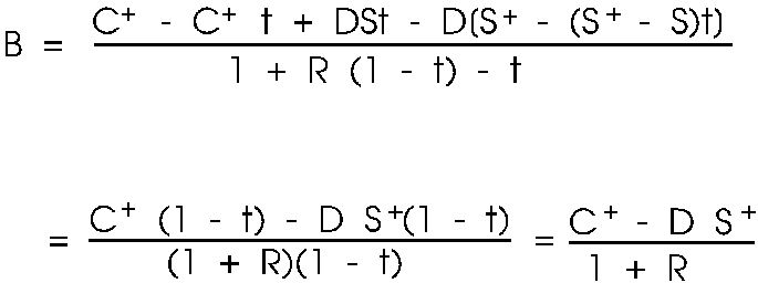
Since C is
D * S = B, this becomes:
 {20}
{20}
Subtracting
one from the other,
 {21}
{21}
so
 {22}
{22}
 {23}
{23}
Equations
{22} and {23} match the old formulas for D and B exactly. Not
only that, but the intrinsic value at expiration is the same no
matter what the tax rate is. While this may seem unintuitive,
no one would ever sell an option for less than intrinsic value,
whether they're getting a piece of their loss back from the government
or not. This means that the value of an option is the same, independent
of the tax rate (given our simplifying assumptions).
Allowing
Non-constant Interest Rates
One of our
assumptions was that the riskless rate was known and constant
over the life of the option. This meant that the yield curve was
flat, and was not going to move at all. We will keep the yield
curve from moving, but will now allow it to have some slope or
curvature.
Given a yield
curve, we can back out the forward rate from any point in the
future to any other point. In building the binomial tree, the
first period is from today (t0) to some point t1 in the future.
The next period goes from t1 to t2, and so on until we go from
tn-1 to tn, where n is the number of periods in the tree and tn
is the expiration of the option. For the first period in the tree,
we should use the forward rate from t0 to t1 as the riskless rate
at which we can borrow and lend. For the next binomial period,
we'll use the forward rate from t1 to t2, and follow this scheme
all the way to expiration.
We will have
an r{sub i} that represents the risk free rate over the ith binomial
period. Now only will we use this rate in our two equations in
two unknowns to borrow and lend, but it will also be important
if we build our up and down moves around the mean return on the
underlying asset, and that mean is a function of the risk free
rate (from the Appendix to "Basic Option Pricing," we
saw that one way to build a tree was to set
{24}
and
where µ
is the annual log mean return on the asset
v is the annual
log standard deviation on the asset
m is the number
of binomial periods per year
This discrete
stochastic process will converge to lognormal diffusion process
(as n approaches infinity) if we set
µ = fr
- v²/2 {25}
where rf is
the one period risk free rate,
v is the one
period log standard deviation of the underlying asset's return.
The proof
of this follows from the Taylor series for e(x) of order 2. It
may be seen intuitively since the binomial tree is multiplicative
and open-ended on the upside, but bounded by zero on the downside.
This means the more periods we have in the tree, the more upward
growth there is. In the limit, with continuous returns, it is
necessary to make the mean of the continuous process lower to
compensate for this, and to make the mean over a finite interval
equal the risk free rate. In actual fact, though, as we add more
periods, this adjustment matters less and less. For the examples
in this paper we ignore it for simplicity.)
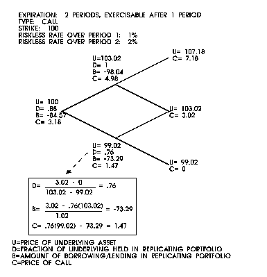
Figure 9 shows
a case where the yield curve is upward sloping.
Figure
9: Upward Sloping Yield Curve Example
Non-constant
Volatility
In every case
so far, we have had trees that grew in size in a linear fashion:
one node became two, two became three, and so on. This is a result
of an up move followed by a down giving the same price as down
and then up. One feature usually necessary for such a non-bushy
tree is that the volatility be constant throughout the life of
the option. For example, if an up move over the first period is
1.05, a down move 1/1.05, and in the second period the moves are
1.08 and 1/1.08, our paths will lead to:
 {26}
{26}
from up down,
and
 {27}
{27}
from a down
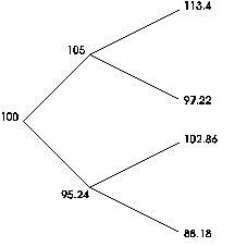
up path. Because these two don't match, we need to build a tree
like the one in Figure 10.
Figure
10: A Bushy Tree
This problem
can become computationally unfeasible very quickly. If a non-bushy
tree with 25 periods takes 1 second to value, a bushy tree with
25 would take over a day, and 50 periods would take 100,000 years!
Clearly, we want to avoid non-bushy trees whenever possible.
When we do
have to use a bushy tree, though, we don't do anything differently,
we just do a lot more of it. We build the tree assuming the asset
can go up or down. Then we work out the intrinsic value at expiration.
Then we work backwards through the tree, solving our two equations
in two unknowns for the value of the replicating portfolio.
There are
times when volatility can appear to be non-constant, and we can
have a non-bushy tree. A great example of this is bonds again.
The price volatility of a bond will decline as it approached maturity.
If we build a tree in yields, as we did before, then convert each
node's yield to a price, the price jumps will be declining in
magnitude as time passes. The price movements will not in general
be a simple function, even if the yield moves are.
SUMMARY
This paper
has extended the basic binomial model presented earlier. It has
discussed how to value puts, American options, American/European
hybrids, options on futures, and forwards. It has also shown how
to value options when there are cash flows on the underlying asset,
a changing strike price, a sloping yield curve, and changing volatility.
Taxes and options on bonds were discussed, as well as put-call
parity. All in all, a lot of ground has been covered. But the binomial
model has proven to be remarkably adept at handling each of these wrinkles.
Once the basic idea is understood, that a portfolio that has the same cash
flows as an asset will have in the future must have the same price as that
asset today, it is very easy to change the equations slightly for each of
the above features. Its simplicity is perhaps its greatest virtue. For
while there may be other methods to value some of the options listed above,
a strong grasp of the binomial will allow one to use it to value options
that don't exist yet, as well.
